Dogs vs Cats – Conclusion

As a final post, I’m going to summarize what I’ve done for this Dogs vs Cats project. Let’s do it chronologically.

Blog post 1: First results reaching 87% accuracy

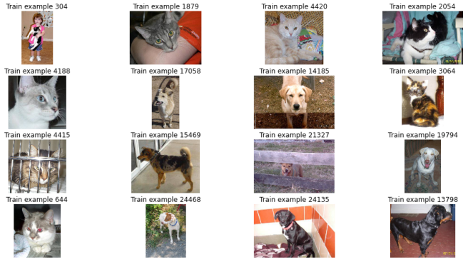
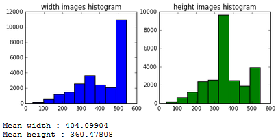
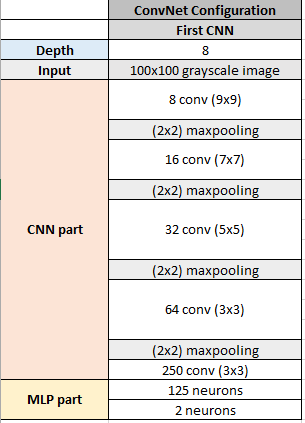
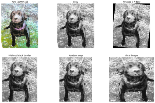
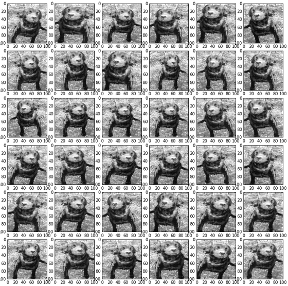
To begin with this project, I started by a relatively small network with an architecture inspired from the very classical AlexNet: a stack of convolutional and 2×2 maxpooling layers, followed by a MLP classifier. The size of  convolutional filters was decreasing as we go deeper into the network: 9×9, 7×7, 5×5, 3×3… ReLUs for each hidden layers and Softmax for the output layer. This network was taking 100×100 grayscale images as inputs. This post also presents quickly my data augmentation pipeline (rotation + cropping + flipping + resizing) which has never changed. This data augmentation process permitted the network to reach an accuracy equal to 87% (without data augmentation, the same network was reaching an accuracy equal to 78%).

Blog post 2:  Adopting the VGG net approach : more layers, smaller filters

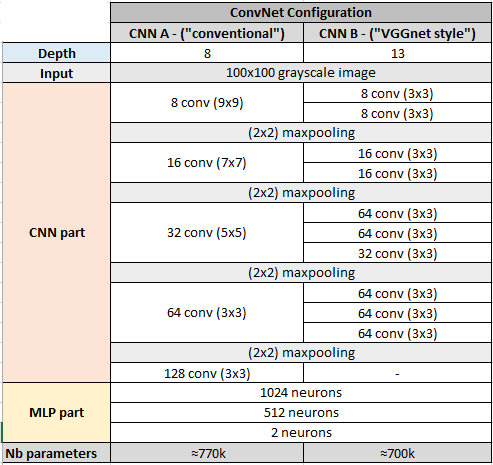
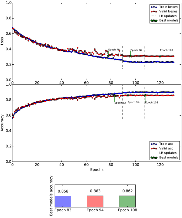
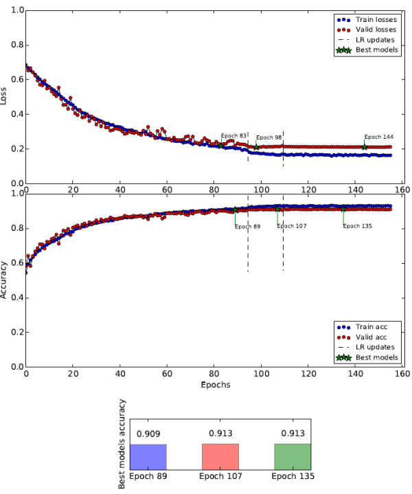
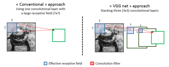
The second post starts by a review of the VGGNet paper. The VGGNet approach consists in increasingly significantly the depth, using only 3×3 convolution filters. In my post, I make a comparison between two models with a comparable number of parameters: one network with an architecture inspired by the VGGNet paper, and another one similar to the network from my first post. The VGGNet-like network won the contest easily: 91% vs 86%. In this post, I started using bigger input image : 150×150, and I’ve used this input size until the end.

Note: All the testset scores reported in the first blog posts (from 2 to 7) corresponds to a score obtained on 2500 trainset images (at this time, I was not aware that it is still possible to make a Kaggle submission after the competition’s end).

Blog post 3: Regularization experiments – 7.4% error rate

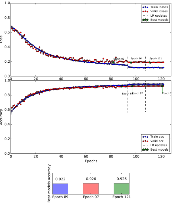
In this post, I presents some regularization experiments. Dropout on fully connected layers permitted me to improve the accuracy of a network presented in the previous post: 92.6% (+1.1%). I also tried weight decay but it was not helping.

Blog post 4: Adding Batch Normalization – 5.1% error rate

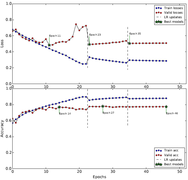
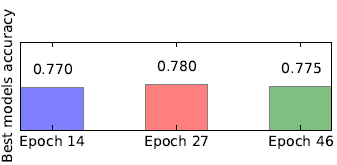
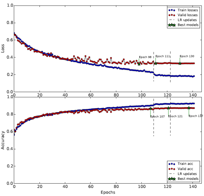
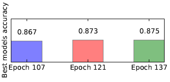
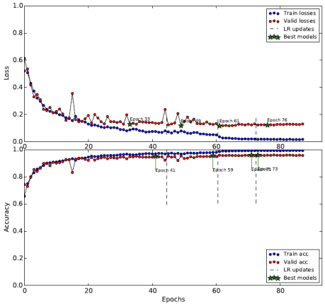
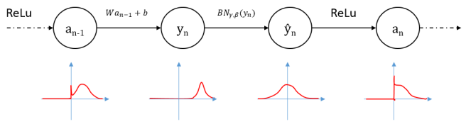
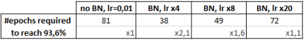
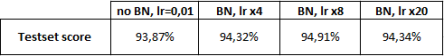
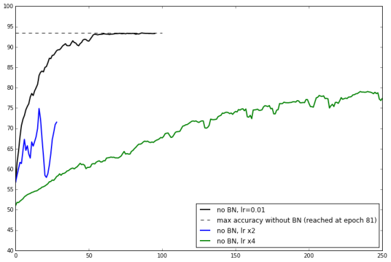
This post starts by a review of the Batch Normalization paper. Batch Normalization is a technique designed to accelerate the training of neural networks by reducing a phenomenon called “Internal Covariate Shift”. It allows the use of higher learning rates, and also acts as a regularizer. After this paper review, I present my experiments when adding Batch Normalization between each layer of my previous network. I verified some claims of the papers: (a) BN accelerates the training: in the best scenario. (b) BN allows higher learning rates: I manage to train a network with a learning rate equal to 0.2. The same model without BN can’t deal with learning rates higher than 0.01. (c) BN acts as a regularizer and possibly makes dropout useless: for me, it turns out that dropout was useless when using BN. (d) BN permits to reach higher performance: with BN, the network reached an accuracy equal to 94.9% (+1% in comparison with the version without BN).

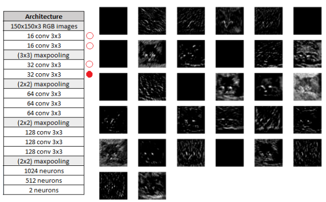
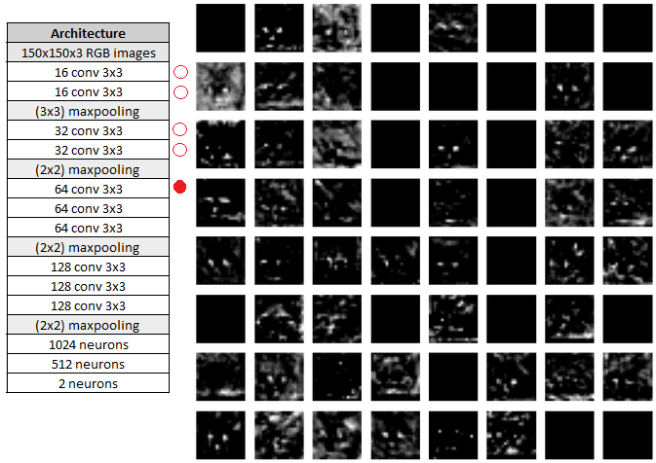
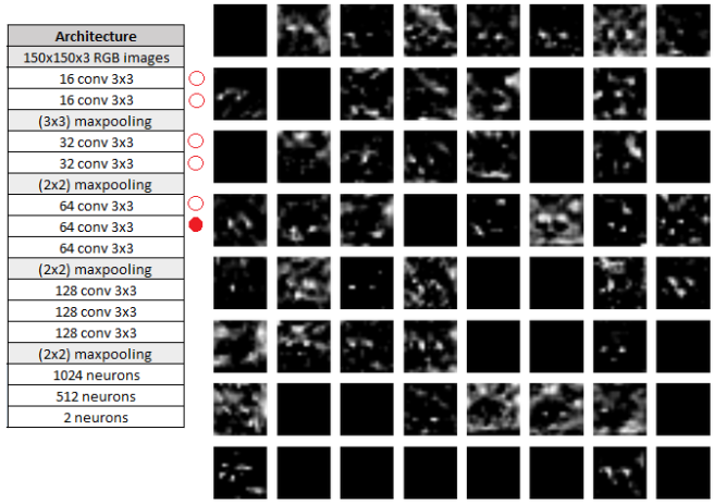
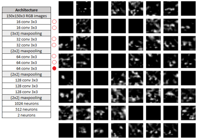
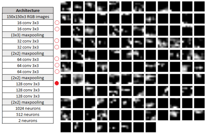
Blog post 5: What’s going on inside my CNN ?

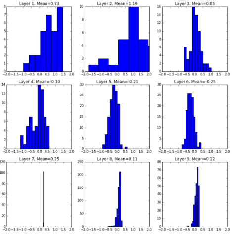
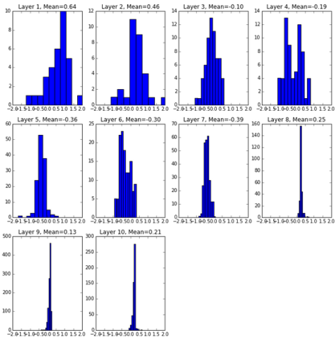
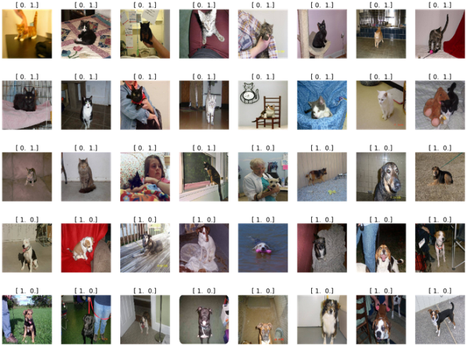
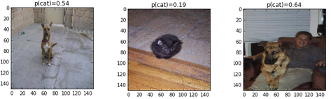
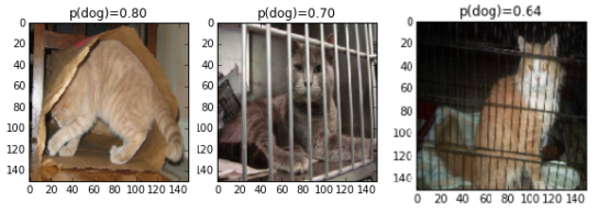
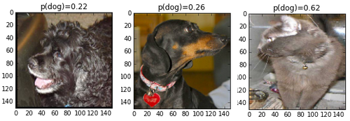
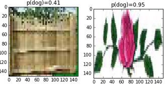
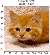
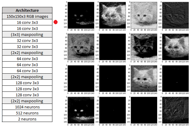
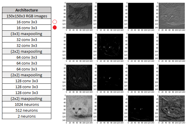
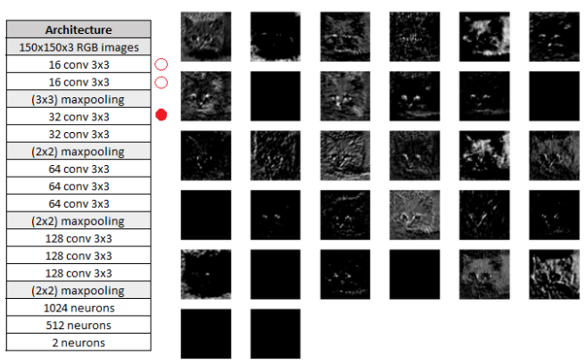
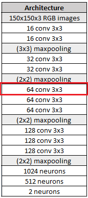
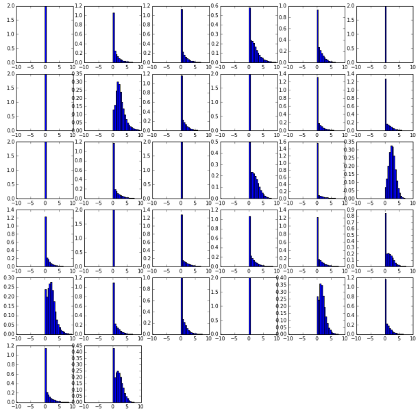
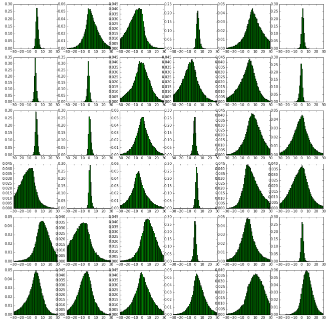
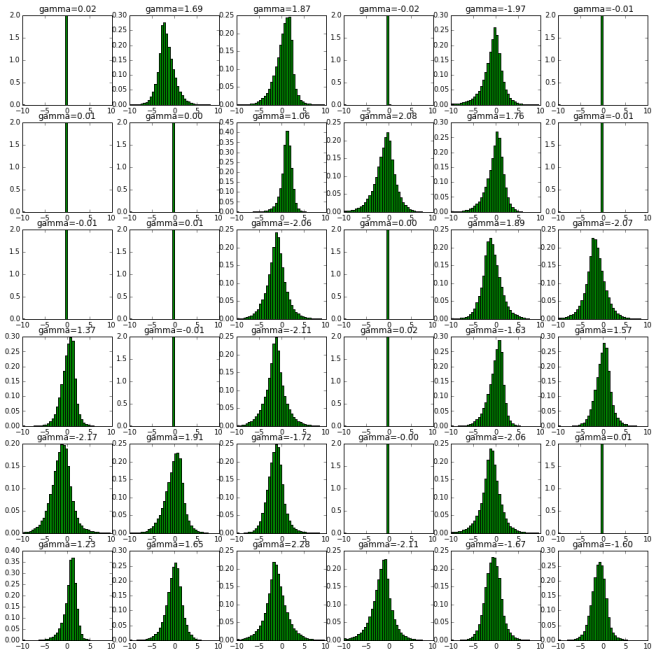
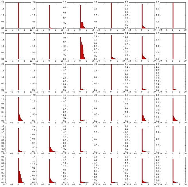
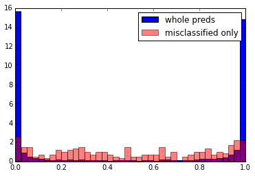
In this post, I decided to spend some time evaluating my best model at this time. I started by an analysis of misclassified images. Then, I showed the feature maps obtained when applying the model on a single example. Finaly, I spent some time describing what’s going on when adding a Batch Normalization in terms of activity distribution.

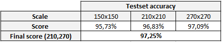
Blog post 6: A scale-invariant approach – 2.5% error rate

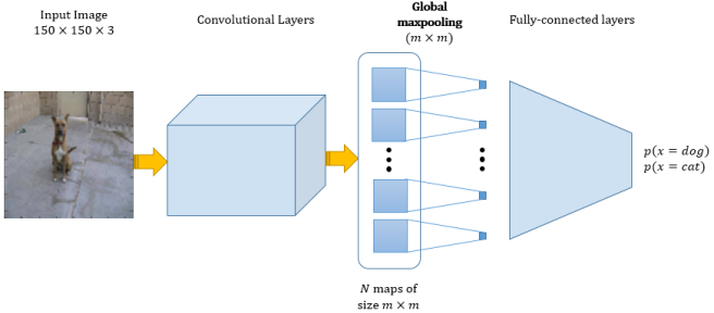
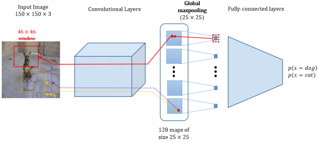
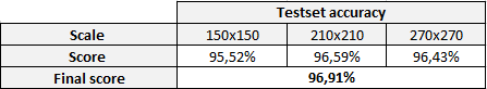
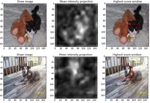
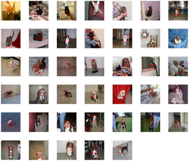
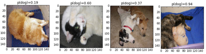
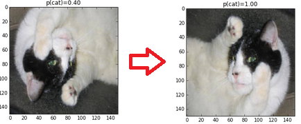
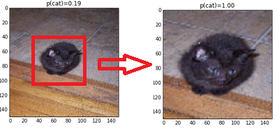
This post presents the kind of architecures that have permitted me to reach really nice results: >97%. This architecture is inspired from this paper: Is object localization for free? by M. Oquab and based on the use of a Global Maxpooling Layer. In this post, I show that this architecture makes the network more scale-invariant, and that the Global Maxpooling Layer absorbs a kind of detection operation. I also showed that the network gives more importance to the head of the pet. In this post, I also presents my new testing approach, which requires averaging 12 predictions per image (varying the input size, the model and flipping or not the image).

Blog post 7: Kaggle submission – Models fusion attempt – Adversarial examples

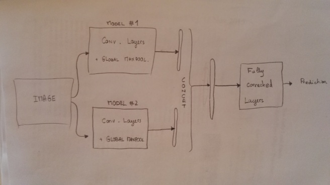
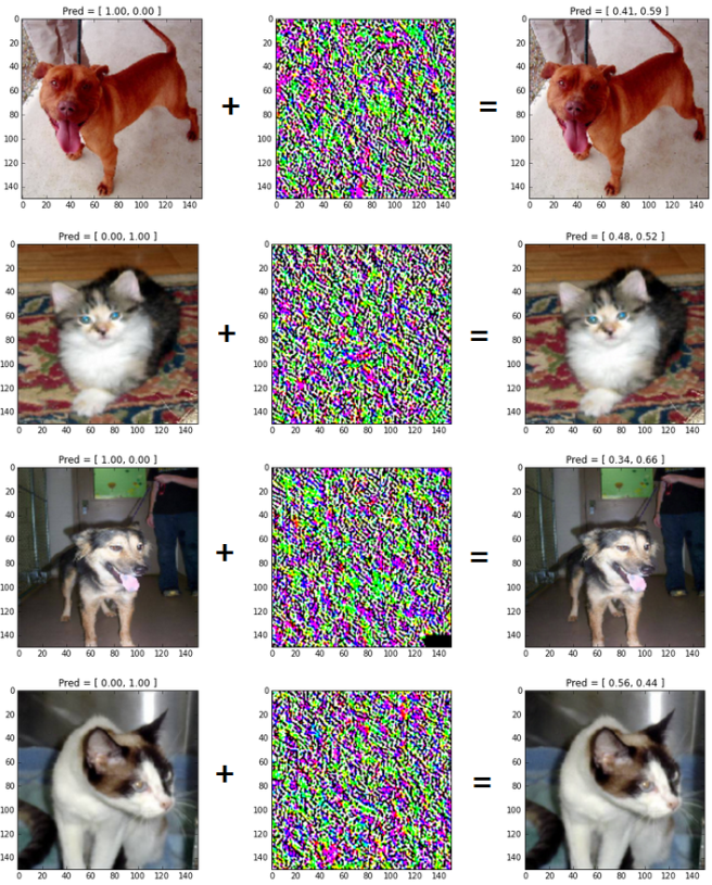
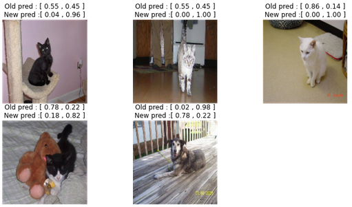
I started this post by showing the Kaggle Testset score (97.51%) obtained by my ensemble of 2 networks presented in the previous post. This score corresponds to my first leaderboard entry. Then, I presented a model fusion attempt: the idea was to concatenate the features outputed by the Global Maxpooling Layer of both models, and give it to a single MLP. This idea has not leaded to higher performance. Finally, I played a bit with adversarial examples (see this paper). In the post, I said that I was working on a way to make my models “robust to adversarial examples by continuously generating adversarial dogs/cats during the training”. It turns out that I’ve never reported my results about that. Let’s do it now: well… it has been a failure… During the training, the network was seeing one batch of “normal” examples, and then one batch containing the corresponding “adversarial examples”. But this approach made the training slower, and at the end, the validationset accuracy was significantly lower (around -1%). But I’ve not played a lot with hyper-parameters for this experiment, so there is maybe a way to make it work.

Blog post 8: Parametric ReLU – 2.1% error rate

In my final post, I describe my experiments when replacing ReLUs by Parametric ReLUs. It improved slightly the Kaggle Testset score: 97.9% (+0.4%). This score corresponds to my second leaderboard entry. Then, as I’ve been asked to clarify some point about my testing approach by classmates, I came back on it. Even if computationally costly, this multi-scale testing approach is one of the main reasons to explain why I  got really good results.

Well… Playing with these dogs and cats was fun. If I had more time, I would have enjoyed trying to implement Spatial Transformer Networks, or experimenting Residual Neural Networks. Maybe next time…

The end.

Dogs vs Cats – Parametric ReLU – 2.1% error rate

Parametric ReLUs

During these last days, I’ve been experimenting an activation function called Parametric ReLU. Similarly to Leaky ReLU, this activation function does not saturate when z < 0. See Figure 1.

Figure 1: (left) ReLU. (right) Parametric ReLU. Figure taken from [1].

PReLUs have been successfully introduced in [1] achieving superhuman performance on the 2015 ImageNet challenge.  The activation function consists in the following operation:

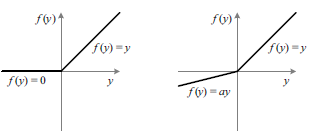
The motivation behind PReLUs is to avoid zero gradients. What makes it different from Leaky ReLU is that is a learnable parameter. When , a PReLU becomes a ReLU. PReLU is therefore a generalization of ReLUs. In terms of complexity, it only adds 1 parameter per channel.

Experiments

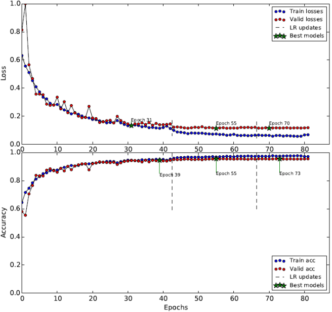
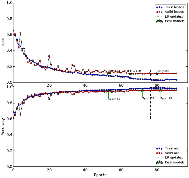
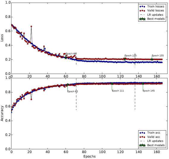
I used exactly the same models as the ones presented in this post (“Window46 and Window100” models). As done in [1], each PReLU parameter (noted above) has been initialized to . Learning curves for each model are displayed in Figure 2 and 3.

Figure 2: Learning curves for the “Window46” model with PReLUs. The final validset score 95.9%.

Figure 3: Learning curves for the “Window46” model. The final validset score is 96.1%.

Testset scores are discussed in the final section.

What has been learned for ?

Let’s take a look at the learned values for . See Figure 4 and 5.

Figure 4: distribution for each layer of Window46.

Figure 5: distribution for each layer of Window100.

Interestingly, for the first layers, the network used various and possibly large  values (from -2.0 to 5.0 for layer 2 of the Window46 model). Deeper layers have smaller values in average. Moreover, for both models, the distribution of the layer just before the Global Maxpooling operation (layer 7 / layer 8) is sharped and centered around 0.25: values have not been updated a lot during the training for these layers. I think this can be explained by the “winner-take-all” phenomenon introduced by the Global Maxpooling Layer which probably makes gradients with respect to  small at this stage (much smaller than for other layers).

Testset scores

As said in my previous posts, my best testset scores have been obtained by averaging many predictions, varying the image size, the model and flipping or not the image. This approach is computationally expensive (12 predictions per image, 6 for each model) but it significantly improves the testset accuracy. When testing only on raw images, I got validset accuracies not far from the ones reported on the leaderboard by my class mates (95.9% for Window46 and 96.1% for Window100). Taking into account the flipped version improves the score by 0.5% in average. Averaging the predictions obtained on 3 different image sizes (150×150, 210×210, 270×270 instead of only 150×150) generally improves the score by more than 1%. Finally, averaging the predictions given by both models improves slightly the score (around 0.3% more).

As can be seen on Figure 6, this costly testing approach permits to reach a decent testset accuracy: 97.91%. This score would have been a top10 result 3 years ago. Of course, I’m using techniques that were not introduced in 2013 (PReLU, Batch Normalization), but my model are quite small (0.6 and 1.7 million parameters only) and we are more constrained that competitors were since we are not allowed to use external data. I’m pretty satisfied by this result.

Figure 6: Testset score obtained by my ensemble of models.

As I’ve been asked by some people this week, let me clarify a point: my models have not been trained in a multi-scale fashion, as Olexa did for instance. During the training, models have always seen 150×150 images. Nevertheless, my data augmentation pipeline involves a random cropping operation which makes the same pet appear at different scale each time it is processed. Moreover, as described in this post, I think that the chosen architecture is somehow scale-invariant and more robust to small pets appearing at random locations. When testing on a bigger image (210×210 or 270×270 for instance), I have to manually adjust the poolsize of the Global Maxpooling layer (see this post for more details about this layer). As said above, averaging predictions for multiple sizes improves significantly the score. For instance, Figure 7 shows the testset score obtained by the Window100 model when averaging 3 predictions per image, corresponding to 3 different image sizes. It already works very well.

Figure 7: Window100 model – Averaging 3 predictions per example: one for each image size (150×150, 210×210, and 270×270). When testing only on 150×150 images, this score is around 96.1%.

Reference:

[1] Delving Deep into Rectifiers: Surpassing Human-Level Performance on ImageNet Classification – He et al, 2015

Dogs vs Cats – Kaggle submission – Models fusion attempt – Adversarial examples

Kaggle Submission:

In my last post, I explained how I managed to reach a testset accuracy equal to 97.5%. Since I was not aware that it is still possible to make a Kaggle submission after the competition deadline, models were trained on 17500 images, validated on 3750 images, and finally tested on 3750 images, with every image taken from the trainset provided on the Kaggle website.  Here is the score when evaluating my ensemble of model on the Kaggle Testset:

Figure 1: Kaggle submission.

I’ve not re-trained my models recently, so I think it is possible to slightly improve this score by using the entire dataset (25000 images) for training & validation.

Models fusion attempt:

The score presented above has been reached by averaging many predictions for each testset images. Varying the image version (raw or left-right flipped), the image size (150×150, 210×210, and 270×270), and the model (Window46 model, and Window100 model), my testing process is arithmetically averaging 12 predictions per testset image. A simple averaging is probably not the optimal way of fusing predictions. With this idea in mind, I tried to fuse models together: just after the global maxpooling operation, features of both models are concatenated and given to the same fully connected block. Figure 2 illustrates the process:

Figure 2: Fusing Window46 and Window100 models together.

Therefore, my Window46 and Window100 models are now sharing the same fully connected layers. Architecture for FC layers: Concatenated features (dim=384) > 1024 neurons > 512 neurons > 2 neurons.

During the training, Conv. layer weights are loaded from my best models (Window46 and Window100 models) and freezed: only the weights from FC layers are learned. I wanted to fine-tune convolutional weights, but I ran into errors when I tried to train the entire network in a end-to-end fashion…

The fused model gives me the following testset accuracy when testing only on 150×150 images:

Note that there is still an averaging going on: Final prediction = Mean (Prediction (raw) + Prediction (flipped)).

And the accuracy when averaging predictions for 3 sizes (150×150, 210×210, 270×270) is:

So, fusing models together has not permitted to reach a higher score. I see two possible reasons to explain it:

• Since only fully connected layers are learned, the training does not make convolutional layers cooperate. Features given by each convolutional block might contain very redundant information.
• The fused model involves less parameters: instead of having 2 fully connected blocks (one for each model) as it was the case when averaging final predictions given by the 2 distinct models, now there is only one. I could have tried to keep the number of parameters fixed by making the FC block of the fused model deeper or wider.

I’ve not pushed further my fusion experiments. I decided to work on something more intriguing and interesting: adversarial examples.

Adversarial examples:

Adversarial examples have been introduced in this paper ([1] Intriguing properties of neural networks, Szegedy et al, 2014).  Citing the abstract, authors have shown that “we can cause the network to misclassify an image by applying a certain hardly perceptible perturbation, which is found by maximizing the network’s prediction error”. See figure 3 for an illustration of adversarial examples obtained for one of my models:

Figure 3: Adversarial examples for my Window46 model.

Following the approach from this other paper about adversarial examples ([2] Explaining and Harnessing Adversarial Examples, Goodfellow et al, 2015), the perturbation has been obtained as:

(code available here)

Adversarial examples shows that the network fails in understanding the true underlying concepts of “Dogs” and “Cats” images. I’m actually trying to make the model robust to adversarial examples by continuously generating adversarial dogs/cats during the training, and adding them to the trainset (as it was done in [1]). These experiments will be reported in my next post.

Dogs vs Cats – A scale-invariant approach – 2.5% error rate

In my last post, I was evaluating the model presented here and I’ve shown some misclassified images. Among them, there were images of small pets appearing at random locations. For those images, an object-detection engine would be beneficial. Unfortunately, we don’t have the ground truth (bounding boxes) to train a detection network. Therefore, I worked on an alternative solution which consists in:

• An architecture which makes the network more scale-invariant. Features used to make the final prediction only depend on small parts of the input image. I’ll show that this network performs a kind of detection operation.
• A multi-scale approach at test time.

By taking profit of these two ideas, I managed to achieve an accuracy of 2.5% on a 3750-images testset by averaging the predictions of two models.

A scale-invariant architecture:

Architectures used in my experiments are inspired by the work presented in this paper: Is object localization for free? by M. Oquab. This article presents a weakly-supervised CNN which accurately predicts both the class and position of objects inside an image, while being trained with class labels only. Therefore, they have shown that it is possible to train a network to detect objects for free (ground truth = labels only).

Figure 1 illustrates the new architecture.

As usual, the network consists in convolutional layers, followed by fully-connected ones. The only difference with conventional architectures is the global maxpooling layer, which is in fact a classical maxpooling with a pooling size equal to the maps’ size of convolutional layers outputs. Therefore, fully-connected layers only see one neuron per final convolutional maps, extracted by the global maxpooling layer. We’ll see later that this global maxpooling layer performs a kind of detection operation (see paragraph “Is detection for free?”). Figure 2 displayed the details of the architecture used in most of my experiments.

Figure 2: Architecture details. 0-padding is used to keep the maps’ size fixed through convolutional layers. Batch Normalization before each non-linearity. SoftMax for the last layer, and ReLu everywhere else. Comparison with the network from my last post: less parameters (630k vs 1m1), and less deep.

Using this architecture, maps outputted by the convolutional part are of size 25×25. Each neuron of these maps only depends on a small part of the input image.  Figure 3 illustrates the situation.

Figure 3: Each neuron outputted by the global maxpooling layer has been influenced by a 46×46 window from the input. Of course, each neuron outputted by the global maxpooling layer has a different corresponding window. The global stride of the convolutional part is equal to 6, so two consecutive input windows are spaced by 6 pixels.

Therefore, after the global maxpooling layer, the network operates on features that have only been influenced by a 46×46 input patch. I think that you can see the convolutional part as a detection engine which scans the input image with sliding windows of size 46×46 searching for some pet components (a “dog head” or a “cat head” for instance). I’ll come back to this idea.

In the rest of the blog post, the model presented above is called “46-window model”.

Multi-scale testing:

Thanks to the global maxpooling operation, I expect the network to be more scale-invariant. But we can make the predictions even more scale-invariant by testing on different input shapes. This approach requires adapting the model to operate on bigger input images:

• 1) Predictions on 150×150 images using the learned model.
• 2) Predictions on 210×210 images: this requires to turn the (25×25) maxpooling into a (35×35) maxpooling. By doing this, the model still scans the input image with 46×46 windows, but since the image is bigger, objects appearing inside those windows are also bigger.
• 3) Predictions on 270×270 images: this requires to turn the (25×25) maxpooling into a (45×45) maxpooling.
• 4) Average the predictions.

46-window model results:

Hyper-parameters used:

• Training examples : 17500
• Validation examples : 3750
• Input : 150×150 RGB images
• Data augmentation : random rotation, and random cropping
• Learning rate : 0.01 first, and it is divided by 10 each time the validation loss stops to decrease (early stopping with patience = 10)
• Momentum : 0.9
• No regularization (except Batch Normalization which can be considered as a regularizer)
• Batch Size = 32

Training curves are shown in Figure 4.

Figure 4: Training curves of the 46-window model.

One epoch takes around 7 minutes on Hadès. The whole training took around 10 hours.

Table 1 displays testset accuracies obtained for each scale, as well as the final score when averaging all predictions.

Table 1 displays testset accuracies obtained for each scale, as well as the final score when averaging all predictions.

When testing on 150×150 images only, the accuracy is equal to 95.5%. Even if the model is far less complex than the one presented in this post (2x less parameters, and less deep), the testset score is increased by 0.6 point. When testing only on 210×210 images, the testset score is even higher: 96.6%. Finally, when averaging predictions done for each scale, the testset accuracy reaches 96.9%.

Note: testset scores displayed above are computing averaging predictions of the raw testset and the flipped testset.

Quick evaluation of the scale-invariance:

To evaluate if the model is really scale-invariant, I manually selected a subset of 40 images containing small pets appearing somewhere in the image. Those 40 images are shown in Figure 5.

Figure 5: Subset of 40 small pets’ images.

Then, I evaluated the 46-window model on this subset, as well as my previous best model. The 46-window model got an accuracy equal to 90.0 % on this subset (only 4 misclassified images), whereas my previous model got an accuracy equal to 77.5 % (9 misclassified images). The 5 images that have been well classified by the 46-window model, but misclassified by my old model are displayed in Figure 6. Even if these scores are computed on a small subset of images, I think that it is honest to consider that the 46-window is more scale-invariant than my previous model.

Figure 7: Images well-classified by the 46-window model, but misclassified by my previous best model.

Is detection for free?

Figure 8 displays something I called the “mean intensity projection”. The mean intensity projection (MIP) is the across-channel mean of the 128 maps outputted by the convolutional part, resized to 150×150. This mean intensity projection gives an approximate answer to the question: what is important inside the input from the network’s point of view? The third subplot displays the window which gave the MIP highest value (the most important window from the network’s point of view).

Figure 8: a) Raw image. b) Mean Intensity Projection maps. c) Most important window according to the network.

By looking at Figure 9, you’ll see that most of the time, this “most important” window is localized near the head of the pet. It seems logical. Therefore, this network could be used as a cheap “head-detection” algorithm.

Figure 9: The “most important” window from the network’s point of view for each image.

 100-window model results:

The 46-window model assumes that the pet can be well described using features only influenced by 46×46 input patches. What happen when increasing the size of the window? I extended my experiments by training a similar network which scans the input image with 100×100 sliding windows spaced by 12 pixels. The architecture is described in Figure 5.

Figure 10: 100-window model architecture. This model has 3x times more parameters, and 2 more non-linearities. The star “*” means that 0-padding is used for this layer.

Training curves are displayed in Figure 6 (same hyper parameters than before).

Figure 10: Training curves of the 100-window model.

And testset scores are given in Table 2 :

Table 1: Testset accuracies of the 100-window model given for each scale, as well as the final score. Predictions from 150×150 images are not used to compute the final score (not helpful).

The 100-window model obtains a better score. It is not a surprise since the model is more complex.

Ensemble of models:

Finaly, I adopted an ensemble approach by averaging predictions of both model for each scale (150,210,270 for 46-window model and 210,270 for 100-window model). This has lead to my best testset score so far : 97.49%.

Plan for future experiments:

• Instead of simply averaging all the predictions, a possible source of improvement can be finding a smarter way to fuse predictions together.
• Searching a solution to improve the score on pets appearing in a strange pose (see my previous post). I think that this is a more difficult problem than making the model more scale-invariant.

Github Repo:

I’ll update my Github repo by the end of the week.

Dogs vs Cats – What’s going on inside my CNN ?

Last Sunday, I presented a model which achieved a testset accuracy of 94.9% (see this post). This network follows the VGG approach (“depth is good”, 3×3 filters), and Batch Normalization is used between each hidden layer. During the last few days, I spent some time trying to understand and visualize what’s going on when using this model. In this post, I’ll present the following stuff :

• Some misclassified images : what kind of images are not well predicted ?
• Intermediate maps : what does the output look like after one convolution ?  after two convolutions ? or after many ones ?
• Closer look at activity distributions : effect of Batch Normalization ?

Misclassified images :

Here are some images that have not been well classified by the model, categorized into classes :

Strange pose/orientation :

The model does not work well when the pet appears in a strange pose. It prefers when the head is in the right direction. For instance, in the case of the second image displayed above, rotating it by 180° makes the prediction good:

Having a network able to automatically rotate the input image with the desired angle would be ideal. In this article, it seems that something like that is done. I’ve planned to read it.

Small pets :

It seems that the model is not scale-invariant enough : when the pet is too small in the image, the prediction is often wrong. In most cases, zooming on the pet makes the model predict well :

Therefore, using a detection engine to first localize and extract the pet in the image would be beneficial.

Partially occluded pets :

I don’t know if there exists a way to make the model more robust to occlusions.

Head in profile :

Also in this case, I don’t know if it is possible to make the model work better on those images, except, of course, adding more “head in profile” images in the trainset.

Fake examples :

It seems that there are some images which do not contain neither a dog nor a cat.

Intermediate maps :

To better understand what’s going on when applying the CNN on an image, I spent some time visualizing intermediate feature maps :

Input Image :

First intermediate maps :

Edges (map 4 and 16), eyes (map 13), textures…

Going deeper…

At this stage, we can still distinguish some part of the cat face : eyes, nose… But features are becoming more and more abstract when going deeper.

From this layer to the end, feature maps are just bright random blobs, and we cannot distinguish any understandable shape.

It is interesting to note that maps are sparse : a lot of activity values are zeros. This must be explained by the use of ReLu (see Deep Sparse Rectifier Neural Network). This sparsity property will be discussed again in next section.

Activity distributions :

Effect of Batch Normalization :

In my last post, I wrote a review of the Batch Normalization paper. A paragraph is dedicated to discuss the fact that performing the normalization before the non-linearity should be more efficient than doing it after. This is due to the fact that distributions are more likely to be smooth and Gaussian after the affine transformation (or convolution operation), and by contrast, distributions might look stange after the non-linearity. The figure below illustrates this point.

I wanted to check this point by plotting the internal distributions of a given layer. I decide to check layer 5 distributions.

Here are the 32 input distributions of layer 5 (one distribution per map, computed using the intermediate outputs of 1000 examples):

There is often a peak at 0, due to the ReLu activation of Layer 4.

After the convolution operation, distributions are smoother : (only 36 distributions over 64 are displayed)

But most of these distrbutions are large, and sometimes shifted. Thanks to Batch Normalization, distribution are brought back around 0 and scaled :

Note : it seems that the network never uses some maps (gamma = 0). This is strange. It is possible that during the training, the optimization process took at some point a path with some gammas equal to 0, and then was not able to get out this situation (?). This point may need further investigation.

Finally, a non-linearity is applied on those normalized distributions :

The last figure is another evidence that feature maps are sparse : high peak at x=0. For this layer, only 25% of neurons are active in average.

Softmax layer :

To conclude this post, I would like to discuss the following figure which displays the activity distribution of the last layer. In fact, only the distribution of the “dog” neuron is displayed, but due to the softmax operation, the distribution of the other neuron is symetrical ().

Activity distribution of the “dog” neuron on the entire testset (blue), when taking into account only misclassified examples (red).

By looking at the blue histogram, we can conclude that most of the time, the network is pretty sure of its predictions : only few examples have a probability of being a dog between 0.1 and 0.9.  On the contrary, when looking at the same distribution computed only on misclassified examples, it looks more uniform. This is a good thing : when the prediction is wrong, the network is most of the time not confident about the answer.

Dogs vs Cats : Adding Batch Normalization – 5.1% error rate

Last tuesday, I did a presentation in IFT6268 class about the Batch Normalization paper. Therefore, I’ll start this blog post by a review of this paper. Then, I’ll present my experiments when adding Batch Normalization layers in a network similar to the one presented in this post.

Batch Normalization

Motivation :

Batch Normalization has been designed to solve a problem called “Internal Covariate Shift”. Although “Internal Covariate Shift” especially affects neural networks, this name comes from a more general Machine Learning problem called “Covariate Shift”. Let’s first see what Covariate Shift is and we’ll come back to Internal Covariate Shift after:

Imagine this situation : a learning system has been trained on a given dataset (ie with a given input distribution) and then, for some reason, the input distribution starts to change. This change of input distribution is a “Covariate Shift”. Since they expect a fixed input distribution, learning systems don’t like Covariate Shifts. As a consequence, parameters of models facing a change of input distribution need to be updated. This situation is a common one in Transfer Learning, or Domain Adaptation.

Now let’s go back to the notion of Internal Covariate Shift, which affects the training of neural networks. Since a neural network is a stack of layers with each of them feeding the next one, the input distribution to a given layer depends on every layers below. Then, something might be problematic when training a neural network with stochastic gradient descent: when you update the parameters of a given layer, you don’t take into account that parameters of previous layers are also going to change, leading to the emergence of Covariate Shifts for each layer of the network. Therefore, the training algorithm needs to continuously adapt the weights to take care of those changes of distribution inside the network. This continuous adaptation has a cost: it slows down the training. Using small learning rates reduces this phenomenon by making small updates to prevent huge change of distributions, but training remains slow. Thus, Internal Covariate Shift is one of the reasons explaining why it is difficult to train very deep networks, for which the Internal Covariate Shift is stronger.

By normalizing internal activations, Batch Normalization is aimed at reducing Internal Covariate Shift.

Batch Normalization operation :

where :

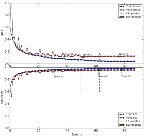
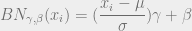
• and are statistics computed for each minibatch during the training :  and . When testing, and a  are statistics computed on the entire trainset.
• and are learnable parameters which allows the network to decide whether or not to normalize. For instance, the setting and can be used to turn off the normalization.

Main benefits :

• It speeds up the training by allowing you to use higher learning rates. For instance, the paper presents experiments in which they took a variant of the GoogLeNet model, and trained it with and without Batch Normalization on the ImageNet dataset. They managed to train Batch Normalization versions with higher learning rates, and for each setting, it reached the same level of performance at least using less steps than required by the version without Batch Normalization (14 times less steps for the fastest setting).
• It acts as a regularizer. Indeed, during the training, the model output for a given example not only depends on the example itself, but also on the other guys which compose the mini-batch. Then, since examples are shuffled at the beginning of each epoch, the same example is going to be seen many times, but each time in a different mini-batch (ie with different and ). And you will ask the model to target the same value each time. I think that you can view it as making the model robust to some noise added on each and . In the paper, they explained that using Batch Normalization permitted to remove dropout in most of their experiments..

Note that in one of their settings, they manage to increase the GoogLeNet variant score (72,2%) by more than 2 points without using dropout, and it took 5 times less steps than required by the GoogLeNet variant to achieve its maximum accuracy. So, it suggests that Bach Normalization can lead to faster and better results.

Discussion :

• I would like to discuss the fact that Batch Normalization should be performed just before the non-linearity, and not just after. After a non-linearity, the activity distribution might look strange. By contrast, after the affine transformation, distributions are more likely to be smooth and Gaussian. The figure below illustrates the situation:

  

  Figure 1: Computational graph of layer n.

  In fact, if you assume that distributions are Gaussian after the affine transformation, then Batch Normalization is going to fully remove Internal Covariate Shift. Indeed, a Gaussian distribution is only parametrized by its mean and variance, and these two statistics are fixed by the Batch Normalization operation. This explains why the article suggests that performing normalization before the non-linearity will be more efficient than doing it after.

• In one of their experiments, they manage to train a deep network using sigmoid activations, despite the well-known difficulty of training such networks. They explained that the same network without Batch Normalization was not able to learn anything. Adding Batch Normalization was the key. To explain this, it is suggested in the paper that Batch Normalization might make gradient propagation better behave. In fact, it is said that “Batch Normalization may lead the layer Jacobians to have singular values close to 1”, which is a good property if you want to train deep networks. But to my knowledge, these claims have not been studied and verified yet, and this seems to be a conjecture. The point here is that Batch Normalization is not fully understood yet, but this technique seems to produce very successfull results.

Dogs vs Cats Experiments :

 I used the network architecture presented in this post, and I doubled each number of feature maps. It resulted in the network presented in Figure 2.

Figure 2: Network architecture. Softmax on the last layer, and Relu everywhere else.

Inspired by the experiments presented in the paper, I tried to reproduce the results provided there by first training a network without BN, and then comparing it with BN versions of the same model. My results are presented in sections below.

Results

Figure 4 shows the evolution of validation accuracy over the training for 4 different models : one trained without BN (red) and three BN models trained with increased learning rates (blue, green, red). Table 1 gives for each model the  number of epochs required to reach 93.6% accuracy (= maximum score of the model without BN). Finally, Table 2 shows Testset scores. Those scores are computed by averaging the predictions given for each testset image and its flipped version (see “Testset scores notes” section).

Figure 3 : Evolution of the validation score over the training for each model.

Table 1 : Number of epochs required to reach the maximum validation accuracy of the model without BN.

Table 2 : Testset score for each model.

Comments for each model :

• No BN, lr = 0.01 : the model without Batch Normalization reached its maximum validation accuracy (93.6%) at epoch 81. The testset score for this model is equal to 93.87%.
• BN, lr x4 : In this case, adding BN and increasing the learning rate to 0.04 leaded to a faster training (this model reached 93.6% at epoch 39) and better performance (+0.45 point compared with the version without BN).
• BN, lr x8 : Same comments. However, although the learning rate is higher, it took more time to achieve an accuracy of 93.6%. This is the best model I managed to train so far (Testset score = 94.9%, +1.05 point compared with the version without BN).
• BN, lr x20 : Same surprising comment : increasing the learning rate has made the training slower. With this learning rate (0.2), the training has not been speeded up by Batch Normalization. At the end, adding BN was still usefull since it increased the testset score by 0.47 point.

Learning rate conclusion :

Here are the validation accuracy curves obtained when training the model without BN with higher learning rates :

Figure 4 : Validation score evolution when training the model without BN with higher learning rates.

Training the model without Batch Normalization using higher learning rates (x2, and x4 here) doesn’t work at all. By contrast, I manage to train the same network with Batch Normalization using much higher learning rates (up to x20). Batch Normalization enables the use of higher learning rates.

Training speed conclusion :

In terms of convergence speed, results here are less impressive than the ones provided in the paper. This might be explained by the fact that, in the paper, they used a deeper network and trained it to perform a much more complicated task. As said in the review section above, deeper is the model, stronger is Internal Covariate Shift. It suggests that Batch Normalization is more usefull when dealing with very deep networks.

Surprisingly (or not ?), experiments above shows that increasing the learning rate does not necessarly mean that the training is going to be faster. On the contrary, increasing further the learning rate causes the model to train somewhat slower. In the paper, they observed the same phenomenon.

Regularization ?

Each model discussed above has been trained without regularization. I tried to add regularization (weight decay, droppout) but it did not help generalization. As the model with BN is concerned, it could mean that the regularization property of BN is enough to reduce overfitting, but I don’t have a good explanation about the fact that regularization doesn’t help in the case of the version without BN.

Testset score note :

Testset scores presented above are computed by averaging the predictions given for each example and its flipped version. This slightly improves the score. For instance, in the case of the “BN, lr x8” model, using the flipped version increased the testset score by 0.75 point.

Dogs vs Cats – Regularization experiments – 7.4% error rate

Well, I spent most of the week working on my code (adding the possibility to use Fuel instead of loading datasets in memory, and moving the scripts to the GPU cluster). But I still have some results about regularization experiments. I took the network presented in my last post (the one taking 150×150 grayscale images), and tried adding some regularizers.

Baseline :

Here are the training curves of the network without regularization:

Figure 1 : Training curve without regularization.

The best model on the validation set obtained the following scores on the testset:

• Testset accuracy : 0.915
• Testset loss : 0.219

Note : in my last post, it is said that this network obtained an accuracy of 92.6%. This result was obtained on a validation set of 5000 examples, after a training over the rest of the dataset (20000 examples). No testset was used. Since showing validset results is a bit dishonest, I now split the dataset in a trainset (17500 examples), a validset (3750 examples) and a testset (3750 examples). So, there is less examples in the trainset now. For this network, this leads to a decrease of 1 point in terms of accuracy. I think it would be interesting making experiments to observe how the accuracy increases with the trainingset size, for a given network. It might be a good way to evaluate the efficiency of a data augmentation operation, which is supposed to compensate the lack of training data.

With regularization :

The objective is to improve performances of the baseline network by adding regularizers. I did the following trials :

• Weight decay (alpha=0.0005)
• Dropout on fully-connected layers (p=0.5)
• Weight decay (alpha = 0.0005) + Dropout on fully-connected layers (p=0.5)
• EDIT : I just got new results with Dropout(p=0.7) on fully connected layers

Testset results are sumarized in the table below :

Figure 2 : Some testset results with different regularizers.

Conclusion :

• Performances are lower when using weight decay.
• Dropout helped a little with p=0.5 (when used alone). EDIT : With a dropping probability of 0.7, the accuracy has been increased by more that 1 point.
• Even if I’ve not done a lot of experiments, I think that for this network and this trainset (17500 grayscale images of size 150×150, with data augmentation described here) regularization is not going to bring a lot. When looking at the baseline training curves, we don’t see much overfitting. I should move to model with higher capacity, taking bigger RGB inputs. EDIT : Well, the new result with “Dropout (p=0.7)” contradicts a little this last statement : adding dropout on fully connected layers permitted to gain more than 1 point.

Best model so far : 

During the week, I figured out that I was using a low momentum : 0.2. So, I increased it to 0.9, and launched the “dropout model” again : it reaches an accuracy of 92.3%, which corresponds to my best result so far. I will start my future experiments with this momentum. EDIT : The best model so far is now the one with Dropout(p=0.7) : accuracy equal to 92.6%. I’ll keep an eye on the momentum value in my next experiments.

Code updates :

As said in the introduction of this post, I’ve spent most of the week working on my code. The main tasks were :

• Adapting my scripts to make them work on Hadès. By the way, this post from Florian Bordes was really helpful.
• Adding the possibility of using Fuel instead of loading datasets in memory (both option are possible now).

I’ll push my code on my GitHub repo during the week-end (probably tomorrow). Feel free to use.

EDIT : my GitHub reo is now up-to-date.

Adopting the VGG net approach : more layers, smaller filters

VGG net :

(VGG = Visual Geometry Group, Department of Engineering Science, University of Oxford)

Few days ago, I read this article which presents the work made by the “VGG” team for the 2014 ImageNet Challenge.

The main contribution of this paper consists in evaluating how increasing depth in CNNs can improve recognition performance. This investigation has been made using deep architectures (from 11 layers to 19) which alternate stacks of convolutional layers with small filters (3×3) and maxpooling layers (2×2). Using this framework, they achieved state-of-the-art results : equivalent to the ones obtained by the GoogLeNet (Szegedy et al. 2014), on the ILSVRC  2014 classification without outside training data.

Processing the input image using a stack of convolutional layers with very small filters was a novel idea. At this time, setting  large receptive fieds (11×11, 9×9, 7×7…) to the first convolutional layers was more conventional. Section 2.3 of the paper is dedicated to a comparison of these two approaches, and can be sumarized as follows :

• The size of the effective receptive field of a N convolutional layers stack with (3×3) filters is equal to ((2N+1) x (2N+ 1)). For instance, a stack of three convolutional layers with (3×3) filters has a (7×7) receptive field with respect to the input image. But, instead of adding only one non-linearity, as it is the case when using a single (7×7) convolutional layer, many non-linearities are introduced (3 in this example). Therefore, the learnt decision function can be more discriminative.
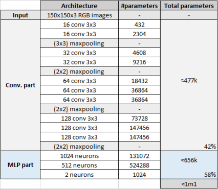
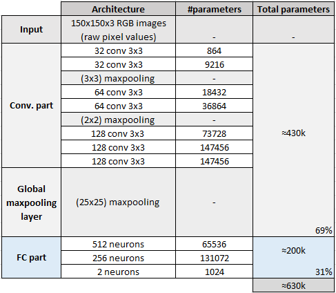
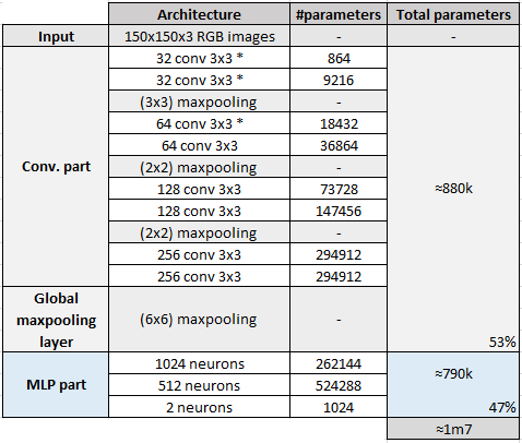
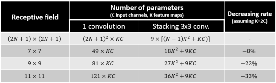• Moreover, for a fixed receptive field, stacking convolutional layers permits to decrease the number of parameters :As can be seen on the above table, increasing depth does not mean necessarly more parameters. For instance, a stack of five convolutional layers with (3×3) filters contains 33% less parameters than a single (11×11) convolutional layer (assuming that the number of feature maps is doubled). Therefore, the authors say : stacking three convolutional layers with (3×3) filters “can be seen as a regularisation on the 7×7 conv. filters, forcing them to have a (3×3) decomposition (with non-linearities injected in between)”.Note : in the article, the demo to show that the number of parameters is decreased when using their approach is done assuming than K is equal to C. This leads to more impressive results, in terms of #parameters decrease. But, to me, the assumption “K = 2C” seems more honest : usually, the number of feature maps increases with depth. In particular, in the rest of the article, they propose architectures where the number of feature maps is always doubled after each stack of convolutions (K = 2C).

 

Dogs vs Cats Experiments :

Then, I decided to test an architecture following the methodology described in this article. More precisely, I decided to compare two networks : one which is similar to the one described in my last post and another one which is deeper and only has (3×3) convolutions. The two architectures are described in the table below :

Notes :

• CNN-A and CNN-B have approximatively the same number of parameters (around 700 000).
• The MLP part configuration is the same for both networks.
• I didn’t try to match the effective receptive field between the two networks. For instance, the receptive field size of the first stack in CNN-B with respect to the input is (5×5), whereas the first convolutional layer in CNN-A is a (9×9) one. The reason is computational : performing convolutions in the first layers is expensive because feature maps are still big at this stage. Stacking many layers before the first maxpooling operation would have significantly increased the computational cost of the whole network.

More details :

• Each activation is a ReLu, except the last one (SoftMax).
• Initial Learning rate : 0.01. Early stopping with patience = 10. At each training stop, the algorithm takes the weights of the best model so far, and re-start the training with a learning rate divided by 10 (see my first post for details), until it reaches 0.0001. In the article, they also use this learning procedure.
• Momentum = 0.2.
• Batch size = 32

Differences with the article :

• No padding (in the article, they use zero-padding to keep the size of maps unchanged).
• The size of feature maps just before the MLP part is (1×1). In the article, this is not the case.
• No dropout, no weight decay : I leave that for future experiments.

 

Results :

Results obtained by CNN-A are displayed below :

CNN-A results : training curves, and accuracy for each “best model”.

CNN-A obtains an accuracy of 86% on the validation set. This result is not far from the one obtained last week during my first experiment (87%).  In the mean time, while having slightly less parameters, CNN-B achieved better performance :

CNN-B improves the accuracy score by 5 points. This experiment shows that : even if keeping an equivalent number of parameters, increasing depth, and adding non-linearities permit to obtain better recognition performance.

Same architecture, bigger input :

This week, I made another experiment : I used almost the same architecture of CNN-B and launched a training taking (150 x 150) grayscale images as inputs. From the architecture described above, I just changed the first (2×2) maxpooling operation to a (3×3) one. By doing this, feature maps just before the MLP part are still of size (1×1). Therefore, the new network takes bigger inputs but still has the same number of parameters. This experiment leaded to a more performant model : > 92% accuracy :

This results is an argument for taking inputs of greater size. But, right now, I’m doing my experiments on my laptop, loading the whole trainset in memory. Taking bigger inputs (or RGB images) is not an option for now. In the future, I plan to use the datastream functionality of Fuel in order to avoid memory errors.

Plan for next experiments :

I think that I’m going to keep the CNN-B architecture for a while, and try to improve recognition performance by adding regularisation  (dropout, weight decay). I also want to try batch normalization.

Dogs vs Cats project – First results reaching 87% accuracy

For the class project, I decided to work on the “Dogs vs Cats” Kaggle challenge, which was held from September 25, 2013 to February 1st, 2014.

Bulldog and Cat Facing Off

Project presentation

The challenge consits in learning a classifier to distinguish cat images from dog ones. A dataset of 25000 pets (12500 cats, and 12500 dogs) is available.

More images (test1) are available on the Kaggle website, but I think (and correct me if I’m wrong) that we don’t have access to the corresponding labels. This testset was used for participant submissions during the challenge.

The winner of this challenge, Pierre Semanet, used external data (CNN pre-trained on ImageNet data) to get 98.9% accuracy. As we are not allowed to use external data, we should obtain less impressive results. Nevertheless, by looking at the leaderboard from last year, I’ve seen that some students managed to obtain more than 97% accuracy without external data, which  are really good results (2 years before, they would have finished in the top 25 of the challenge).

Quick look at the data

First, we can observe that images differ in size. Moreover, dogs and cats appear in random location, pose, and are sometimes occluded. This will not facilitate the classification task.

Concerning the size distribution, here are some statistics :

First CNN :

In order to avoid any potential memory error for this first experiment, I decided to work with 100 x 100 grayscale images. It means that almost all images from the dataset are downsampled (see histograms above).

I used the architecture displayed on the table below :

The networks consists in :

• 4 convolution layers each followed  by a 2×2 maxpooling
• A last convolution layer to bring 3×3 feature maps to 1×1 features maps (or neurons). At this stage, each feature has seen the whole input image.
• A MLP with one hidden layer of 125 neurons, and one output layer of size 2, with SoftMax activation.

The number of feature maps increases with depth while filter sizes decrease with depth. I used ReLu every where, except for the last layer which has a SoftMax activation.

Results without data augmentation :

I divided the dataset into a trainset of 20000 examples, and a validationset of 5000 examples. I first tried to train the network without data augmentation, and I got the following results.

Let me give some explanations on those curves :

• I used Early Stopping to decide when to stop the training. But when the stop criterion is fulfilled (validation loss has not decreased for 10 epochs), I re-loaded the best model (in terms of accuracy), and launch a new training loop from here with a smaller learning rate (divided by 10). I do it until the learning rate is below a certain lower bound. For this experiment, I started from a learning rate equal to 0.01 and the training hasn’t ended until it was smaller than 0.0001. On the curves, each vertical line corresponds to a learning rate update. By doing this, my idea was to maybe improve a little bit the best model, and get closer to a local minima.
• We can observe that the model begins to overfit quickly (at epoch 11). At epoch 22, the first early stopping criterion was reached. Then, the algorithm loaded the weights from the best model so far in terms of accuracy (model from epoch 14) and started a new training from here, with a learning rate equal to 0.001. At epoch 35, the learning rate has been updated again, and a training loop started from the model obtained at epoch 27. At the end, this process permitted to gain 1 point in terms of accuracy (model from epoch 27) on the validationset :

Note : the gain of 1 point between epoch 14 and epoch 27 is only relevant for the validationset. Since I didn’t have a testset for this experiment, I can’t be sure that the learning rate procedure used here was usefull.

In conclusion, without data augmentation, the CNN got an accuracy of 78%. Since we are asked to obtain 80% in a first time, this result is already not so far. Let’s now look at the performances obtained with data augmentation.

Results with data augmentation :

Here are the curves obtained with data augmentation, following the procedure described in the last part :  (data augmentation operations are presented in the next paragraph)

Accuracy is now around 87% on the validationset.

Data augmentation operations :

Raw images are randomly rotated (-10 degrees < angle < 10 degrees), cropped (crop size < 10% of the image size) and left-right reversed with a 50% probability. The process is summarized in the figure below :

The figure below shows the same dog image processed by the random preprocessing 36 times :

Library used and hardware :

For these experiments, I used the Keras library :

Keras is a minimalist, highly modular neural networks library, written in Python and capable of running on top of either TensorFlow or Theano. It was developed with a focus on enabling fast experimentation. Being able to go from idea to result with the least possible delay is key to doing good research.

Description taken from here.

Experiments were done on my laptop’s GPU, which is a Nvidia Geforce GTX 850M (640 CUDA cores, 2 Go).  For this architecture, one epoch takes around 50 seconds (with batch size = 32).

My code is not already on my GitHub repo, but it will be done by tomorrow.

EDIT : my code is now available on GitHub. I tried to explain how it should be used in a README file, but you can send my an email if it is not clear.

Plan for the next days :

• First, I would like to try other architectures (more features maps, more layers, and maybe smaller filters, as it is done here). I also want to move to color images and increase the size of the input.
• I want to compare the learning rate procedure used here with an algorithm like ADAM which adapts the learning rate for each parameter during the training.
• I also plan to test some input normalization techniques (ZCA whitening for instance), and regularization ones (weight decay, dropout…).

 

 

Theano Tutorial

Since we are going to work with Theano most of the time, I started a tutorial this week.

Some notes and code lines are available in this ipython notebook. For instance, the notebook contains the code of a theano implementation of linear regression (taken from theano slides presented in class)  and logistic regression  :

Linear Regression

Logistic regression